
Airline Safety
Health insurance is a type of insurance that helps pay for medical expenses. It works by pooling resources and spreading the financial risk associated with major medical expenses across the entire population to protect those who require medical attention. Whether purchased privately or funded by the government, medical insurance is essential to provide protection against increasing medical costs. The Affordable Care Act of 2010 was designed to extend health insurance to those who could not afford it; however, costs continue to grow.
With the cost of healthcare in the country today, the need for health insurance is stressed and overemphasized. An individual essentially needs health insurance to maximize their savings on healthcare. One of the biggest issues plaguing health insurance is its high cost, which cannot be directly calculated by individuals beforehand. There are many factors that drive the increasing costs of health insurance, some of which are directly related to the personal attributes of the policy holder. Our project is aimed to determine which personal attributes contribute most toward health insurance costs and use regression models to predict the cost based on these attributes.
We obtained Medical Cost Personal Dataset from Kaggle that contained 1338 records of insured individuals, each providing information about the following variables:
the age of the policy holder, ranging from 18 to 64 with the mean age of 39
a binary variable indicating whether the policy holder is male (M) or female (F), contains 676 males and 662 females
the body mass index of the policy holder, ranging from 15.96 to 53.13 with a mean BMI of 30.66
the number of children insured through the insurance policy, ranging from 0 to 5, with a mean of 1
a binary variable indicating whether the policy holder smokes (yes) or not (no), contains 274 that smoke and 1064 that do not smoke
indicates where the policy holder resides: 324 from the northeast, 325 from the northwest, 364 from the southeast, and 325 from the southwest
the cost of health insurance in dollars, ranging from $1121.87 to $63770.43 with a mean of $13270.42
We converted the binary variables, sex and smoker, into binary labels, where female=0 and male=1 and no=0 and yes=1. We also converted the regions into encoded labels, where northeast=0, northwest=1, southeast=2, and southwest=3. We transformed the BMI variable from a continuous variable into encoded labels by binning the values into the following categories, as provided by the CDC:
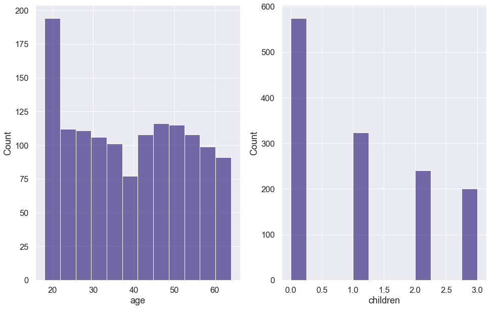
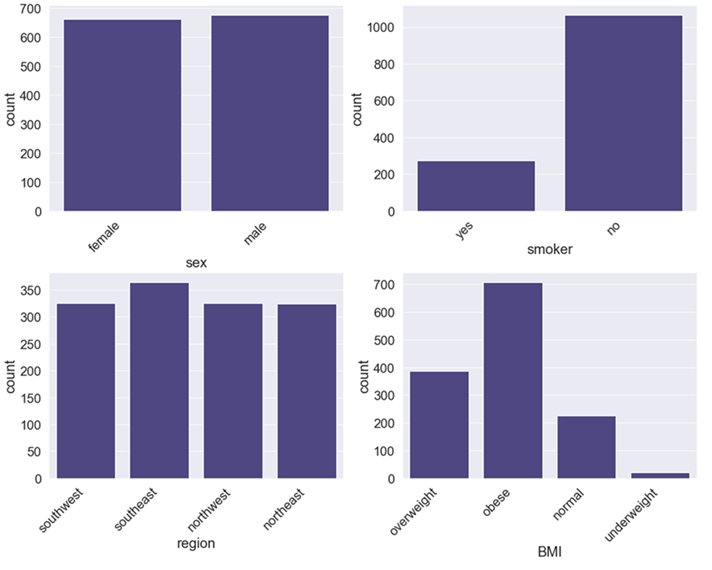
The data contained records with 20 underweight BMIs, 225 normal BMIs, 386 overweight BMIs, and 707 obese BMIs. Finally, many insurance companies only charge for a maximum of three children, requiring no additional fee if more than three children are on the policy. As a result, we combined observations with 4 and 5 children with those of 3. The children variable can be thought of as a categorical variable, where children=3 represents "3 or more" children. The final breakdown of value counts was: 574 with 0 children, 324 with 1 child, 240 with 2 children, and 200 with 3 or more children. After preparing our data, we created histograms of our numerical variables, as seen in Figure 1, and bar plots of our categorical variables, as seen in Figure 2.
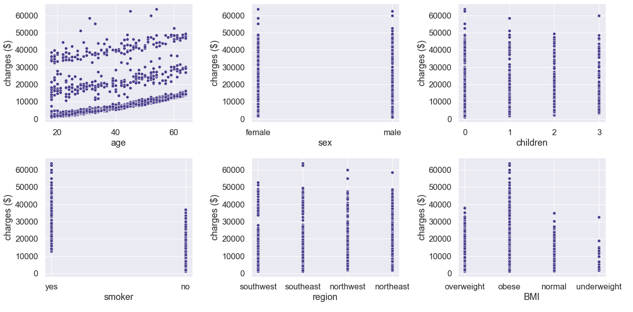
We also created scatterplots of the variables against charges, as seen in Figure 3. Based on the scatterplots, we observed there were three distinct groups of charges by age, with each group having slightly increasing charges as age increased. Charges appeared to be greater for policy holders that smoke and have increased BMIs. The charges by gender, number of children, and region appeared to be consistent.
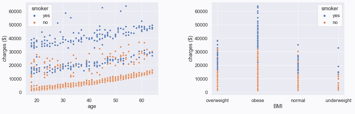
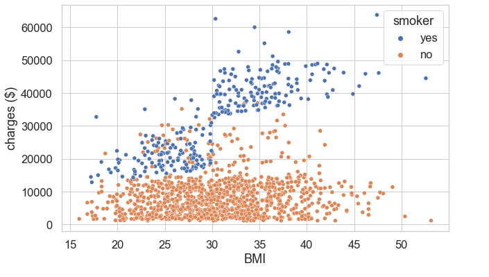
We created modified scatterplots by removed these three variables and included the smoker variable as a third variable, as seen in Figure 4. Based on these scatterplots, we observed that those who smoke are generally charged more, regardless of their age. We also observed that those who both smoke and have higher BMIs are charged more. We looked at BMI as it originally appeared in the dataset, as a continuous variable, and noticed a linear relationship between BMI and charges for smokers, as seen in Figure 5.
Looking at the data, it appeared the most significant variables contributing to health insurance charges were age, BMI, and whether the policy holder smoked or not. However, we used a decision tree regression model to determine feature importance. First, we split our data into training, validation, and test sets, with the training set containing 50% of the data and the remaining 50% split evenly between the validation and test sets. Next, we trained the decision tree regression model on our training data, with BMI in categorical form. The results were as follows:
| Variable | smoker | BMI | age | children | region | sex |
|---|---|---|---|---|---|---|
| Significance | 62.3% | 16.5% | 15.3% | 2.9% | 1.6% | 1.4% |
We repeated the process but with BMI as a continuous variable as it originally appeared in the data. The results were as follows:
| Variable | smoker | BMI | age | children | region | sex |
|---|---|---|---|---|---|---|
| Significance | 61.9% | 20.9% | 13.8% | 1.6% | 1.1% | 0.8% |
BMI as a continuous variable has more significance than as a categorical variable. It also lessens the significance of region, children, and sex. Therefore, we selected smoker, BMI as a continuous variable, and age as the variables to use in our regression models.
Using the selected variables – smoker, BMI, and age – we trained and fit linear regression, decision tree, and random forest models to the validation data. We decided to use the R-squared and mean absolute error metrics to evaluate the performance of our models. R-squared is a statistical measure that represents the proportion of the variance for a dependent variable that is explained by an independent variable or variables in a regression model. Whereas correlation explains the strength of the relationship between an independent and dependent variable, R-squared explains to what extent the variance of one variable explains the variance of the second variable. The mean absolute error (MAE) measures the average magnitude of the errors in a set of forecasts, without considering their direction. It measures accuracy for continuous variables. Using these metrics to evaluate the models, we obtained the following results:
| Model | R-squared | MAE |
|---|---|---|
| Linear Regression | 0.708 | 4163.34 |
| Decision Tree | 0.683 | 3239.07 |
| Random Forest | 0.780 | 2833.14 |
The random forest regression model performed better than the other two models. Next, we concatenated our training and validation data and performed a cross-validation grid search to choose the hyper-parameters for our random forest regression model. Using the grid search to find the values that resulted in the best mean absolute error score, the following parameters were selected:
Using these parameters, we trained the random forest with the training and validation data and fit it on our test data. We obtained an R-square of 0.86 and MAE of 2022.03. The results using the fine-tuned random forest shows increased performance in both performance metrics. The resulting R-squared value indicates that 86% of our data fit the random forest regression model. The mean absolute error indicts our prediction is off by $2022.03 on average.
Based on the regression models we used, we saw improved prediction when using the fine-tuned random forest model. However, there may be other models that increase prediction performance. Our analysis and predictions were limited to the variables in our dataset. There are many other factors that may contribute to the costs of health insurance, besides the personal attributes of the policy holder. Some of these factors may include, but are not limited to, the following:
Airline Safety

Disneyland Review Analysis

Credit Card Churn

Credit Card Churn

Health Insurance Cost
I would love to hear from you.