
Airline Safety
Breast cancer is the most common type of cancer among women – 1 in 8 women in the United States will be diagnosed at some point in their life. Mammographic images are used to detect abnormal masses in breast tissue. Based on the observed attributes of the mass, a physician may recommend a biopsy to determine a diagnosis. A fine needle aspiration (FNA) biopsy is a common form of the procedure, in which a physician uses a needle attached to a syringe to withdraw tissue or fluid from the mass. Mammographic images and FNA biopsies tend to have diagnosis inaccuracies, yielding false negative rate of 20% and 12%, respectively. False negative, or Type II, diagnosis results are the most damaging as they allow breast cancer to remain undetected and treatment to be delayed. Delays in treatment increase the risk of metastasis, which can reduce life expectancy. I will use the Haberman’s Survival dataset to determine which variables are most significant to the survival of a patient. I will use the Mammographic Imaging and Biopsy datasets to determine which variables are most significant to predict breast cancer with high accuracy and perfect recall, avoiding any false negative predictions. This will ensure breast cancer does not go undetected and increases survival.
Using different datasets, I will answer the following questions:
All datasets were obtained from Kaggle.com and include the following information:
age of the patient at the time of surgery
year the surgery was performed
number of positive axillary lymph nodes
status of the patient 5 years post-surgery, where 1 = survived and 2 = died
standard system used to describe findings where:
age of patient
shape of the mass, where
description of the mass’s edge, where
density of the mass, where
diagnosis of the mass, where 0 = benign and 1 = malignant
mean of distances from the center of the cell nuclei to the points on its perimeter
mean texture of the nuclei, described by the spatial arrangement and variation of grey values observed
mean distance around the nuclei
mean area of the nuclei
mean of the local variation in radius lengths
diagnosis of the mass, where 0 = malignant and 1 = benign
For each dataset, I performed exploratory data analysis. I examined the variables to find which are the most significant in predicting breast cancer and the survival of a patient. I used different classification models to identify which provides the best accuracy and recall in predicting a diagnosis.
How My Approach Addresses the Problem
Type II errors, or false negatives, allow breast cancer to remain undetected and treatment to be delayed. Delays in treatment increase the risk of metastasis, or the spread of cancer to other parts of the body, which can reduce life expectancy. I used the survival data to determine which variables contribute most to the survival of a patient. I used the data from mammographic images and fine needle aspiration biopsies to determine how to predict breast cancer with high accuracy and perfect recall to ensure breast cancer does not go undetected and increase the chance of survival.
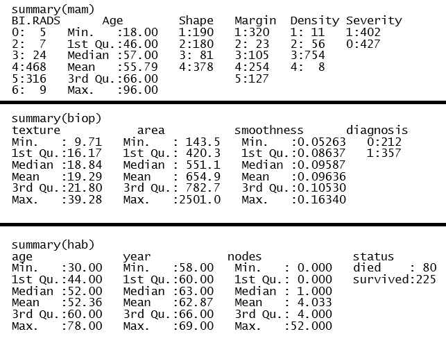
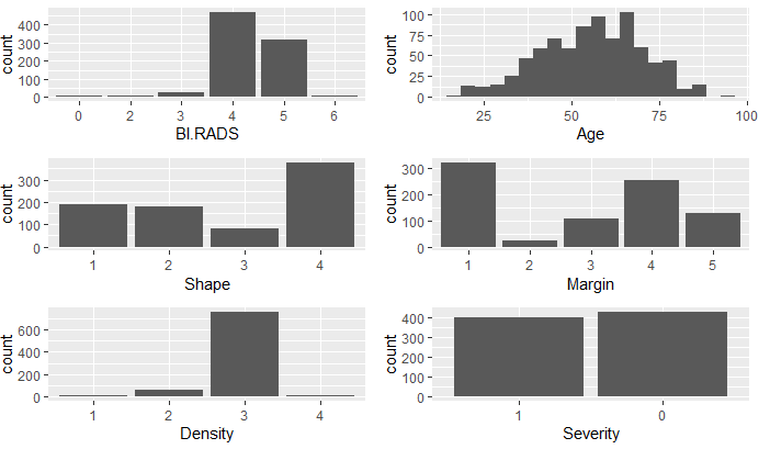
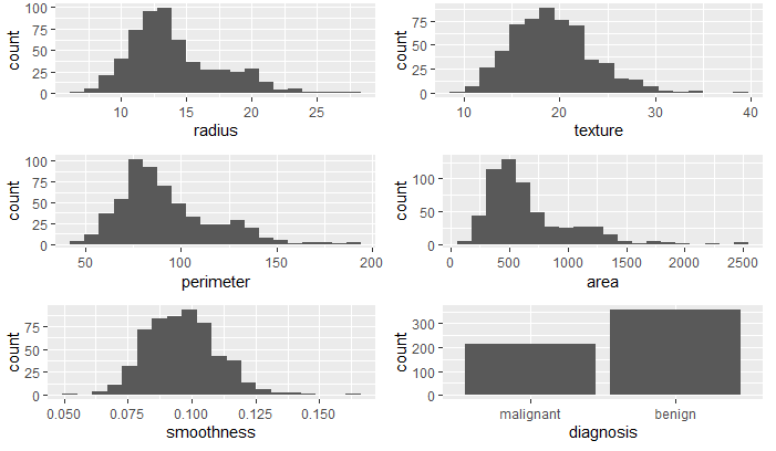
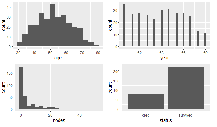
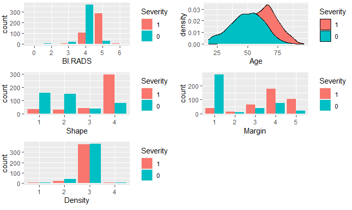
First, I imported each dataset and looked at the structure and data summary for each. In doing so, I verified no missing data. The summary of the mammographic mass dataset showed an observation that had a value of 55 for BI.RADS. As BI.RADS is an ordinal, categorical variable, I have removed this observations from the dataset. No other outliers were evident in the datasets. I converted categorical variables, indicating ordinal variables where appropriate. The summaries of the clean datasets can be seen in Figure 1 and the variable distributions can be seen in Figures 2 - 4. The variables in the biop and hab datasets have skewed-right distributions.
First, I determined which variables were significant in determining the survival status. I compared the variables between the two groups, died and survived, and use density and boxplots for visual aids.
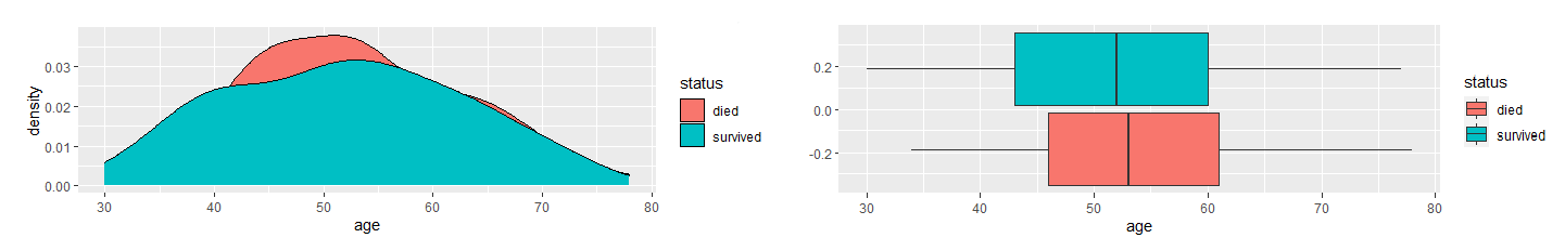
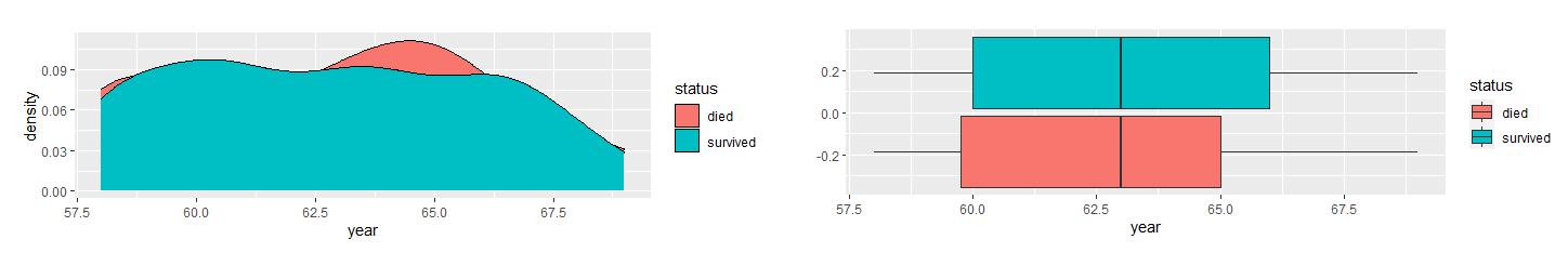
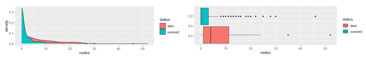
Based on the density and boxplots, it appeared the only significant variable is nodes. As the variables are skewed-right, I used the Mann-Whitney U Test to verify this claim.
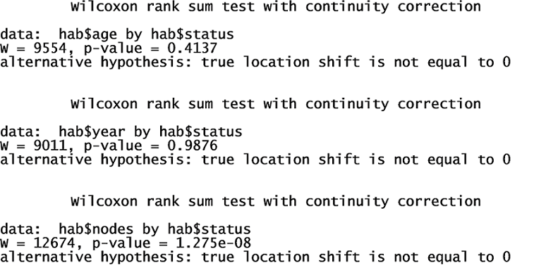
The results showed that there is a significant difference in nodes between the two groups. They also indicated that there is no difference in age and year. Therefore, I concluded nodes is the only significant factor in the dataset in determining whether a patient will survive longer than five years after breast cancer surgery.
To determine which variables are significant in determining the diagnosis of breast cancer, I compared the variables between the two groups, malignant and benign, and use density and boxplots for visual aids.
It appeared that all variables, except Density, are significant variables in predicting Severity. To decide which variables to use in the logistic model, I used all variables in the dataset to determine the most significant. The full model summary indicated age, shape, and margin are the most significant.
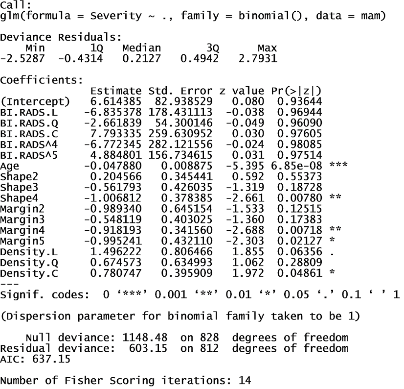
I used these variables in a new logistic regression model. The AIC is much lower, which indicates this model is a better fit than the full model.
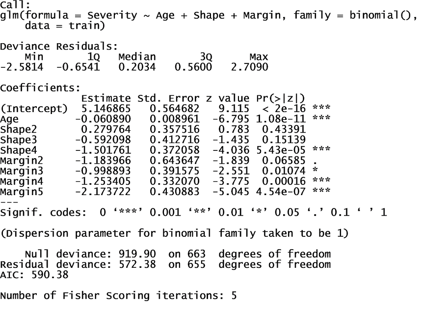
I trained the model using training data and ran the test data through the model. Using a decision threshold of 50%, the model provided a prediction accuracy of 80% and a recall of 79%. To eliminate Type II Errors, I decided to decrease the decision threshold to a value that produced 100% recall. Using a decision threshold of 6%, the model provided a prediction accuracy of 58.2% but 100% recall. The full decision tree model indicated BI.RADS, age, shape, and margin are the most significant variables, as seen below.
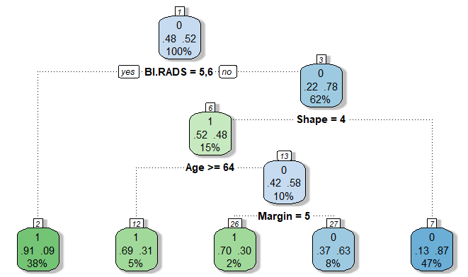
Using the training and testing data, the decision tree model provided a prediction accuracy of 83.6% and a recall of 79.8%. The k-nearest neighbors model, when k = 29, provided a prediction accuracy of 80% and a recall of 85%. Using cross validation on a random forest model, BI.RADS was indicated as the only significant variable. The random forest model provided a prediction accuracy of 81.8% and a recall of 84.7%. The decision tree model provided the most prediction accuracy; however, the best model is the logistic regression model with decision threshold of 6% with 100% recall, as seen in Table 1.
| Model | accuracy | recall |
|---|---|---|
| Logistic Regression | 80.0% | 79.0% |
| Logistic Regresion - 6% threshold | 58.2% | 100% |
| Decision Tree | 83.6% | 79.8% |
| k-Nearest Neighbors | 80.0% | 85.0% |
| Random Forest | 81.8% | 84.7% |
To decide how to proceed with the radius, perimeter, and area variables, I used scatterplots to examine the relationship between them.
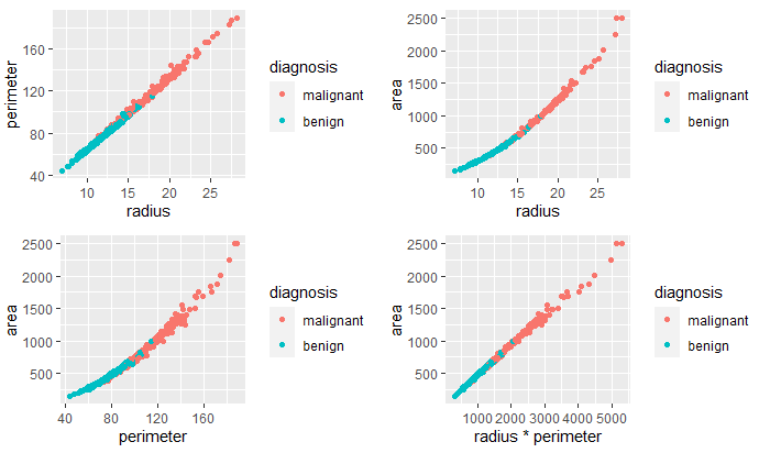
The variables are highly correlated, as suspected. To help decide which two variables to remove from the data frame, I examined their correlation coefficients.
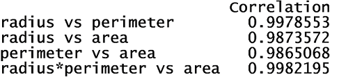
The greatest correlation was between the product of the radius and perimeter variables and the area variable. Therefore, I removed the radius and perimeter variables. Next, I examined the correlation between the remaining variables.
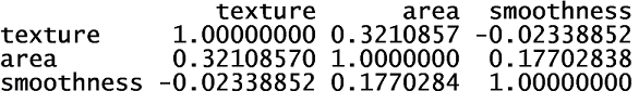
None of the remaining variables were highly correlated with the others. Next, I compared the variables between the two diagnosis groups, malignant and benign. I used density and boxplots for visual aids.
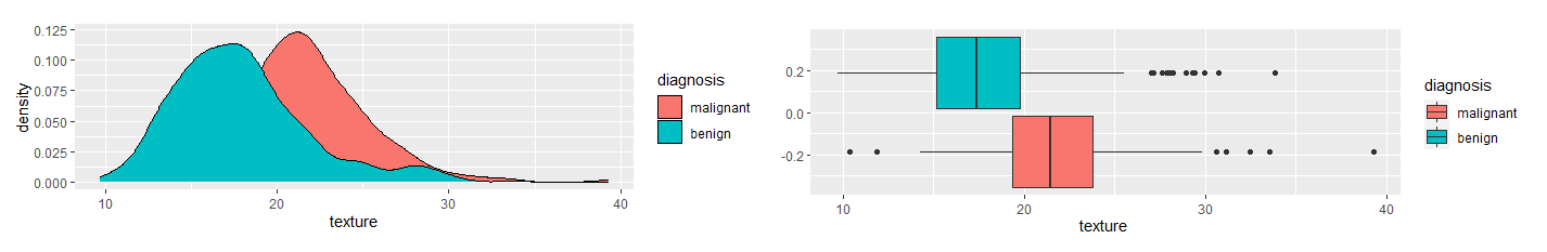
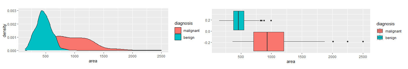
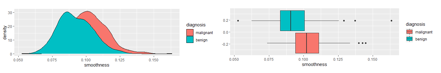
Based on the density and boxplots, it appeared there was a significant difference in texture, area, and smoothness between the two diagnosis groups. I used the Mann-Whitney U Test to show verify.
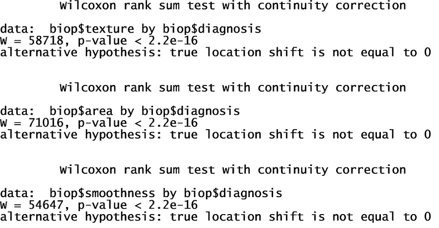
The Mann-Whitney U Test verified these claims. Therefore, I used these variables in a logistic regression model. I trained the model using training data and ran the test data through the models. Using a 50% decision threshold, the logistic regression model provided a prediction accuracy of 92% and a recall of 86.7%. To eliminate Type II Errors, I decreased the decision threshold to 26%. This provides a prediction accuracy of 94.7% and 100% recall. The decision tree model provides a prediction accuracy of 90.3% and a recall of 83%. The k-nearest neighbors model, when k = 23, provides a prediction accuracy of 86.7% and a recall of 71.4%. The random forest model provides a prediction accuracy of 92.9% and a recall of 90.5%. The logistic regression model with a 26% decision threshold provides the best prediction accuracy with perfect recall. Table 2 provides a summary of these results.
| Model | accuracy | recall |
|---|---|---|
| Logistic Regression | 92.0% | 86.7% |
| Logistic Regresion - 26% threshold | 94.7% | 100% |
| Decision Tree | 90.3% | 83.0% |
| k-Nearest Neighbors | 86.7% | 71.4% |
| Random Forest | 92.9% | 90.5% |
The only variable found to be significant in predicting the survival of a patient was the number of positive axillary lymph nodes. Axillary lymph nodes are taken from the axilla, or the armpit. When cancer cells are detected in the axillary lymph nodes, it indicates metastasis. As observed in the analysis, smaller amounts of positive lymph node increased the probability of surviving for longer than five years after surgery. These finding emphasizes the importance of recall accuracy, early detection, and timely treatment. The best recall results were obtained by decreasing the decision threshold in the logistic regression models. There may similar methods available to use on the other classification models; however, time limitations did not allow for further methods to be explored. The survival analysis conducted were based on data gathered from patients who had surgery between 1958 to 1970. Using current data would likely produce different results. I used this data to find the classification models that predicted a diagnosis with high accuracy and recall. As breast cancer continues to affect so many, I feel further research into risk factors associated with its development would provide some interesting insights. These insights could decrease false negative results and increase survival.
By adjusting the decision threshold, I was able to obtain 100% recall using logistic regression with the mammographic and biopsy datasets – resulting in no false negative diagnosis. The prediction accuracy using the mammography dataset was only 58.2%, which would require biopsies for many women with false positive results. However, the prediction accuracy using the biopsy dataset was 94.7%.
Airline Safety

Disneyland Review Analysis

Credit Card Churn

Credit Card Churn

Health Insurance Cost
I would love to hear from you.